Formal multi-product break-even-analysis
by Clemens Werkmeister
Explicit formal analysis of the multi-product case
Break-even-analyses for multi-product cases have to deal with joint fixed costs for several products, and variable costs, fixed costs and sales revenues that can be linked directly to the products. Measuring the multiple products by a single index is one way to solve the problem; allocating (joint) fixed costs to the different products is another way.
Such simplifications are useful ways to deal with complex problems in many situations but sometimes simple approaches neglect critical information and exclude useful solutions. A more sophisticated solution can make the difference in a competitive environment. At least, the more sophisticated solution serves as a benchmark and allows both quantitative and qualitative assessments of other approaches. We introduce the explicit analysis of the multi-product case in the following steps:
- Analysis of the case of two products with joint fixed costs
- Analysis of the case of two products with joint and individual fixed costs
- Analysis of the two-product case with capacity restrictions
- Analysis of the multi-product case with capacity restrictions.
A detailed analysis of theses cases is available in Schweitzer/Troßmann (1998) and Schweitzer/Troßmann/Lawson (1992).
The case of two products with joint fixed costs
If we know constant unit prices (p1, p2) and unit variable costs (kv1, kv2) for two products, and the joint fixed costs (Kf) necessary for their production, we can put the break-even-condition with respect to the production volumes (x1, x2) in the following way:
- E = K = p1 · x1 + p2 · x2 = kv1 · x1 + kv2 · x2 + Kf
Using unit contributions d1 and d2 respectively, and rearranging results in:
- Kf = (p1-kv1) · x1 + (p2-kv2) · x2 = d1 · x1 + d2 · x2
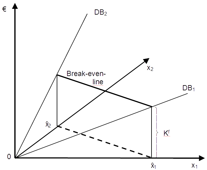
It is obvious that the contribution to be achieved with one product depends on the contribution provided by the other product. In extreme cases, we concentrate on one of the products and set the volume of the other equal to zero. This leads to the individual break-even-points (or break-even-corner-points):
- x1* = Kf/d1 (if x2 = 0)
- x2* = Kf/d2 (if x1 = 0)
Since we assumed linear cost-volume-profit-relations (due to the constant unit prices and variable costs), a 50/50-combination of x1* and x2* will cover the fixed costs too. This can be easily seen for x1 = 0.5· x1* and x2 = 0.5 · x2*:
- d1 · x1 + d2 · x2 = d1 · 0.5 · x1* + d2 · 0.5 · x2* = d1 · 0.5 · Kf/d1 + d2 · 0.5 * Kf/d2 = Kf.
Other linear combinations enable fixed-cost-coverage in a similar way. Together, the corresponding break-even-points build a straight line between the break-even-corner-points, the break-even-line, as can be seen in the following three-dimensional graph (with x1 and x2 as horizontal axes and the profit, contribution and costs at the vertical axis.
In order to facilitate algebraic formulations, we introduce the price vector (p1, p2), the variable cost vector (kv1, kv2), the unit contribution vector (d1, d2) and the output vector (x1, x2). The break-even-line is defined by the following output vector:
The case of two products with individual and joint fixed costs
Sometimes, cost-volume-profit analysis has to cope both with individual and joint fixed costs. Typical examples are multi-stage production processes: Computers are often manufactured for global customers in a single plant (with joint fixed costs) and customized to local specifications (power plugs, manuals, packaging, …) in local facilities. Movie production requires a large joint cost block to get the director’s cut, but finishing, translating, synchronization, subtitles and marketing are done separately for different countries or languages and cause individual fixed costs.
In our two-product case, we introduce Kf1 and Kf2 to capture the individual fixed costs of products 1 and 2 and get the following break-even-form:
- (p1-kv1) · x1 + (p2-kv2) · x2 = d1 · x1 + d2 · x2 ≥ Kf + Kf1 + Kf2
Obviously, we only accept output-quantities x1 and x2 that cover their individual fixed costs. Thus, the individual break-even-conditions hold too:
- d1 · x1 ≥ Kf1
- d2 · x2 ≥ Kf2
This results in the condition:
- x1 ≥ x1 = Kf/d1
- x2 ≥ x1 = Kf/d2
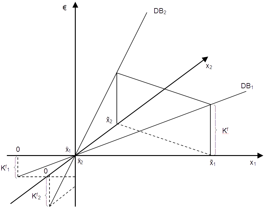
The solution of the two individual conditions results in two break-even-points x1* and x2*. Considering for the joint fixed cost leads to two break-even-corner-points x1** and x2**. The possible break-even-points lie on the line between these corner-points. The graphical presentation of this case is similar to the previous case without individual fixed costs. However, we adjust the horizontal axes (x1 and x2) for the volumes that are necessary to cover the individual fixed costs.
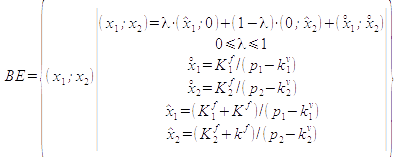
In a formal way this break-even-line is captured by the set:
Note, that different to the previous case without individual fixed costs (and different to the formula proposed in Schweitzer/Troßmann (1998, p. 177), in this case the set of break-even-points is not just a linear combination of the two break-even-corner-points x1** and x2**. Instead, it still is a linear combination of the break-even-points x1* and x2*, corresponding to the joint fixed costs, plus the quantities x1* and x2* to cover the individual fixed costs.


