Formal multi-product break-even-analysis: Unterschied zwischen den Versionen
(Die Seite wurde neu angelegt: „''by Clemens Werkmeister'' <html><img src=""http://vg06.met.vgwort.de/na/c7a3898531b948bb8f88a959a26e3156"" width=""1"" height=""1"" alt=""""></html> == Explic…“) |
Keine Bearbeitungszusammenfassung |
||
| (8 dazwischenliegende Versionen desselben Benutzers werden nicht angezeigt) | |||
| Zeile 1: | Zeile 1: | ||
''by Clemens Werkmeister'' | ''by Clemens Werkmeister'' | ||
<html><img src= | <html><img src="http://vg06.met.vgwort.de/na/c7a3898531b948bb8f88a959a26e3156" width="1" height="1" alt=""></html> | ||
== Explicit formal analysis of the multi-product case == | == Explicit formal analysis of the multi-product case == | ||
[[Break-even-Analyse|Break-even-analyses]] for [[Multi-product break-even-analysis|multi-product]] cases have to deal with joint fixed costs for several products, and variable costs, fixed costs and sales revenues that can be linked directly to the products. Measuring | [[Break-even-Analyse|Break-even-analyses]] for [[Multi-product break-even-analysis|multi-product]] cases have to deal with joint fixed costs for several products (or '''common fixed costs'''), and variable costs, fixed costs and sales revenues that can be linked directly to the products '''(direct costs)'''. Measuring multiple products by a single index is one way to solve the problem; allocating (joint) fixed costs to the different products is another way.<br> | ||
Such simplifications are useful ways to deal with complex problems in many situations but sometimes simple approaches neglect critical information and exclude useful solutions. A more sophisticated solution can make the difference in a competitive environment. At least, the more sophisticated solution serves as a benchmark and allows both quantitative and qualitative assessments of other approaches. We introduce the explicit analysis of the multi-product case in the following steps:<br> | Such simplifications are useful ways to deal with complex problems in many situations but sometimes simple approaches neglect critical information and exclude useful solutions. A more sophisticated solution can make the difference in a competitive environment. At least, the more sophisticated solution serves as a benchmark and allows both quantitative and qualitative assessments of other approaches. We introduce the explicit analysis of the multi-product case in the following steps:<br> | ||
* Analysis of the case of two products with joint fixed costs | * Analysis of the case of two products with joint (or common) fixed costs | ||
* Analysis of the case of two products with joint and individual fixed costs | * Analysis of the case of two products with joint and individual (or direct) fixed costs | ||
* Analysis of the two-product case with capacity restrictions | * Analysis of the two-product case with capacity restrictions | ||
* Analysis of the multi-product case with capacity restrictions. | * Analysis of the multi-product case with capacity restrictions. | ||
A detailed analysis of theses cases is available in Schweitzer/Troßmann (1998) and Schweitzer/Troßmann/Lawson (1992).<br> | A detailed analysis of theses cases is available in Schweitzer/Troßmann (1998) and Schweitzer/Troßmann/Lawson (1992). The [[Accounting exercises 4: Break-even-Analysis|exercise pages]] offer useful examples.<br> | ||
| Zeile 23: | Zeile 23: | ||
Using '''unit contributions''' d<sub>1</sub> and d<sub>2</sub> respectively, and rearranging results in:<br> | Using '''unit contributions''' d<sub>1</sub> and d<sub>2</sub> respectively, and rearranging results in:<br> | ||
: K<sup>f</sup> = (p<sub>1</sub>-k<sup>v</sup><sub>1</sub>) · x<sub>1</sub> + (p<sub>2</sub>-k<sup>v</sup><sub>2</sub>) · x<sub>2</sub> = d<sub>1</sub> · x<sub>1</sub> + d<sub>2</sub> · x<sub>2</sub><br> | : K<sup>f</sup> = (p<sub>1</sub>-k<sup>v</sup><sub>1</sub>) · x<sub>1</sub> + (p<sub>2</sub>-k<sup>v</sup><sub>2</sub>) · x<sub>2</sub> = d<sub>1</sub> · x<sub>1</sub> + d<sub>2</sub> · x<sub>2</sub><br> | ||
It is obvious that the contribution to be achieved with one product depends on the contribution provided by the other product. In extreme cases, we concentrate on one of the products and set the | It is obvious that the contribution to be achieved with one product depends on the contribution provided by the other product. In extreme cases, we concentrate on one of the products and set the number of units of the other equal to zero. This leads to the '''individual break-even-points''' (or '''break-even-corner-points'''):<br> | ||
: | |||
: | : [[Datei:x_hat_1.png]] = K<sup>f</sup>/d<sub>1</sub> (if x<sub>2</sub> = 0)<br> | ||
Since we assumed '''linear cost-volume-profit-relations''' (due to the constant unit prices and variable costs), a 50/50-combination of | : [[Datei:x_hat_2.png]] = K<sup>f</sup>/d<sub>2</sub> (if x<sub>1</sub> = 0)<br> | ||
: d<sub>1</sub> · x<sub>1</sub> + d<sub>2</sub> · x<sub>2</sub> = d<sub>1</sub> · 0.5 · | |||
Since we assumed '''linear cost-volume-profit-relations''' (due to the constant unit prices and variable costs), a 50/50-combination of [[Datei:x_hat_1.png]] and [[Datei:x_hat_2.png]] will cover the fixed costs too. This can be easily seen for x<sub>1</sub> = 0.5 · [[Datei:x_hat_1.png]] and x<sub>2</sub> = 0.5 · [[Datei:x_hat_2.png]]: <br> | |||
: d<sub>1</sub> · x<sub>1</sub> + d<sub>2</sub> · x<sub>2</sub> = d<sub>1</sub> · 0.5 ·[[Datei:x_hat_1.png]] + d<sub>2</sub> · 0.5 · [[Datei:x_hat_2.png]] = d<sub>1</sub> · 0.5 · K<sup>f</sup>/d<sub>1</sub> + d<sub>2</sub> · 0.5 · K<sup>f</sup>/d<sub>2</sub> = K<sup>f</sup>.<br> | |||
Other linear combinations enable fixed-cost-coverage in a similar way. Together, the corresponding break-even-points build a straight line between the break-even-corner-points, the '''break-even-line,''' as can be seen in the following three-dimensional graph (with x<sub>1</sub> and x<sub>2</sub> as horizontal axes and the profit, contribution and costs at the vertical axis.<br> | Other linear combinations enable fixed-cost-coverage in a similar way. Together, the corresponding break-even-points build a straight line between the break-even-corner-points, the '''break-even-line,''' as can be seen in the following three-dimensional graph (with x<sub>1</sub> and x<sub>2</sub> as horizontal axes and the profit, contribution and costs at the vertical axis.<br> | ||
[[Datei:break-even-line.png]] | [[Datei:break-even-line.png|thumb|left]]<br> | ||
<br style="clear:left;"/> | |||
In order to facilitate algebraic formulations, we introduce the price vector (p<sub>1</sub>, p<sub>2</sub>), the variable cost vector (k<sup>v</sup><sub>1</sub>, k<sup>v</sup><sub>2</sub>), the unit contribution vector (d<sub>1</sub>, d<sub>2</sub>) and the output vector (x<sub>1</sub>, x<sub>2</sub>). The break-even-line is defined by the following output vector: | In order to facilitate algebraic formulations, we introduce the price vector (p<sub>1</sub>, p<sub>2</sub>), the variable cost vector (k<sup>v</sup><sub>1</sub>, k<sup>v</sup><sub>2</sub>), the unit contribution vector (d<sub>1</sub>, d<sub>2</sub>) and the output vector (x<sub>1</sub>, x<sub>2</sub>). The break-even-line is defined by the following output vector: | ||
: [[Datei:break-even-line-set.png]] | : [[Datei:break-even-line-set.png]]<br> | ||
==The case of two products with individual and joint fixed costs== | ==The case of two products with individual and joint fixed costs== | ||
Sometimes, cost-volume-profit analysis has to cope both with individual and joint fixed costs. Typical examples are '''multi-stage production processes''': Computers are often manufactured for global customers in a single plant (with joint fixed costs) and customized to local specifications (power plugs, manuals, packaging, …) in local facilities. Movie production requires a large joint cost block to get the director’s cut, but finishing, translating, synchronization, subtitles and marketing are done separately for different countries or languages and cause individual fixed costs. <br> | Sometimes, cost-volume-profit analysis has to cope both with individual and joint fixed costs. Typical examples are '''multi-stage production processes''': Computers are often manufactured for global customers in a single plant (with joint fixed costs) and customized to local specifications (power plugs, manuals, packaging, …) in local facilities. Movie production requires a large joint cost block to get the director’s cut, but finishing, translating, synchronization, subtitles and marketing are done separately for different countries or languages and cause individual fixed costs. <br> | ||
In our two-product case, we introduce K<sup>f</sup><sub>1</sub> and K<sup>f</sup><sub>2</sub> to capture the individual fixed costs of products 1 and 2 and get the following break-even-form:<br> | In our two-product case, we introduce K<sup>f</sup><sub>1</sub> and K<sup>f</sup><sub>2</sub> to capture the individual (or direct) fixed costs of products 1 and 2 and get the following break-even-form:<br> | ||
: (p<sub>1</sub>-k<sup>v</sup><sub>1</sub>) · x<sub>1</sub> + (p<sub>2</sub>-k<sup>v</sup><sub>2</sub>) · x<sub>2</sub> = d<sub>1</sub> · x<sub>1</sub> + d<sub>2</sub> · x<sub>2</sub> ≥ K<sup>f</sup> + K<sup>f</sup><sub>1</sub> + K<sup>f</sup><sub>2</sub><br> | : (p<sub>1</sub>-k<sup>v</sup><sub>1</sub>) · x<sub>1</sub> + (p<sub>2</sub>-k<sup>v</sup><sub>2</sub>) · x<sub>2</sub> = d<sub>1</sub> · x<sub>1</sub> + d<sub>2</sub> · x<sub>2</sub> ≥ K<sup>f</sup> + K<sup>f</sup><sub>1</sub> + K<sup>f</sup><sub>2</sub><br> | ||
| Zeile 51: | Zeile 54: | ||
: x<sub>2</sub> ≥ x<sub>1</sub> = K<sup>f</sup>/d<sub>2</sub> <br> | : x<sub>2</sub> ≥ x<sub>1</sub> = K<sup>f</sup>/d<sub>2</sub> <br> | ||
The solution of the two individual conditions results in two break-even-points | The solution of the two individual conditions results in two break-even-points [[Datei:x_circle_1.png]] and [[Datei:x_circle_2.png]]. Considering too for the joint fixed cost leads to two break-even-corner-points [[Datei:x_tilde_1.png]] and [[Datei:x_tilde_1.png]]. The possible break-even-points lie on the line between these corner-points. The graphical presentation of this case is similar to the previous case without individual fixed costs. However, we adjust the horizontal axes (x<sub>1</sub> and x<sub>2</sub>) for the units that are necessary to cover the individual fixed costs.<br> | ||
[[Datei:break-even-line-both.png|thumb|left]]<br> | |||
<br style="clear:left;"/> | |||
In a formal way this '''break-even-line''' is captured by the set:<br> | In a formal way this '''break-even-line''' is captured by the set:<br> | ||
| Zeile 59: | Zeile 64: | ||
: [[Datei:break-even-line-joint-set.png]] | : [[Datei:break-even-line-joint-set.png]] | ||
Note, that different to the previous case without individual fixed costs (and different to the formula proposed in Schweitzer/Troßmann (1998, p. 177), in this case the set of break-even-points is not just a linear combination of the two break-even-corner-points x<sub> | Note, that different to the previous case without individual fixed costs (and different to the formula proposed in Schweitzer/Troßmann (1998, p. 177), in this case the set of break-even-points is not just a linear combination of the two break-even-corner-points[[Datei:x_tilde_1.png]] and [[Datei:x_tilde_2.png]]. Instead, it still is a linear combination of the break-even-points [[Datei:x_hat_1.png]] and [[Datei:x_hat_1.png]], corresponding to the joint fixed costs, plus the units [[Datei:x_circle_1.png]] and [[Datei:x_circle_2.png]] necessary to cover the individual fixed costs.<br> | ||
== Analysis of the two-product case with restrictions== | |||
If our production process suffers from limited capacity (for example limited availability of inputs, limited market demand for some products, and so on), not all of the points on the break-even-line presented in the unrestricted case are feasible. For our product analysis it is important whether each product has a specific capacity constraint (individual restrictions) or whether one or several capacity constraints affect several products simultaneously (joint restrictions). <br> | |||
Individual restrictions are rather easy to handle. A direct restriction B<sub>j</sub> to the volume of product j (caused for example by limited market size) can be amended to the break-even-line-set. The same is possible if we face an indirect constraint B<sub>ij</sub> of factor i (for example skilled labour) for product j. In this case, a production coefficient a<sub>ij</sub> can capture the relation between product volume and necessary labor. The corresponding restrictions are:<br> | |||
: x<sub>j</sub> ≤ B<sub>j</sub> or <br> | |||
: x<sub>j</sub> ≤ B<sub>j</sub>/a<sub>ij</sub>.<br> | |||
To be sure, for a<sub>ij</sub> = 1, the former case is the same as the latter.<br> | |||
Joint restrictions are more difficult to handle. They occur if several products need the same, limited input factors or try to sell at the same market. In the linear case, with limitational production factors, the sum of inputs i needed for the several products j has to stay below the available capacity B<sub>i</sub>. Since this is the general case which covers the former cases with direct or indirect product-specific restrictions too, the set of break-even-points is given just for this case. | |||
Using vector notation for the capacity restraint, he set of break-even-points is: <br> | |||
: [[Datei:break-even-set-joint-restrictions.png]]<br> | |||
== The multi-product case == | |||
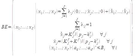
Since we are familiar with the two-product case, it is straightforward to generalize it to the multi-product case with n products (j = 1, …, J). Using again the unit prices p<sub>j</sub>, the variable costs k<sup>v</sup><sub>j</sub>, the product-related fixed costs K<sup>f</sup><sub>j</sub> and joint fixed costs K<sup>f</sup>, and the capacity constraints B<sub>i</sub> and production coefficients a<sub>ij</sub>, we get the following set of break-even-points in the multi-product case with joint restrictions.<br> | |||
: | |||
[[Datei:break-even-multi-product-general-set.png ]] | |||
A break-even-line consists of the possible quantities of two products which cover joint fixed costs and linear sales revenue and variable cost functions. In the case of three products we get a '''break-even-plane.''' The combinations of four or more products result in '''break-even-hyper-planes''' which are difficult to present graphically. For such cases, the analysis is restricted to the vector form of the set of break-even-points (as presented above; and in more detail by Schweitzer/Troßmann (1998, pp. 173 ff.; 203 ff.) or Schweitzer/Troßmann/Lawson (1992), Chapter 4).<br> | |||
== Evaluation of explicit multi-product break-even-analyses == | |||
A large number of managerial decisions deal with multi-product or similar problems (for example product or regional market differentiation, or aiming at economies of scope). They combine both individual and joint production processes, and hence, cost. In many cases, the exact outputs of those products or volumes of the markets are unknown. Thus, a break-even-model that provides information about critical outputs or market volumes, is useful. Break-even-corner-points and intuitive graphical representations of the cost-volume-profit-problem support the decision making processes and [[Controlling|controlling]] and offer valuable additional information compared to the simplifying use of single-product or single-index break-even approaches. However, the more products we include in the analysis, the more contingent are our break-even-hyper-planes. Whether a certain quantity of a product is sufficient or not, depends on the outputs of (too) many other products. In such situations, other approaches may provide better guidelines for decision-making. Apart from the simplifying break-even-analyses already mentioned, this could be the identification of typical output combinations and the calculation of their profit.<br> | |||
---<br/> | |||
References:<br/> | |||
[[Break-even-Analyse]]<br> | |||
[[Multi-product break-even-analysis]]<br> | |||
[[Accounting exercises 4: Break-even-Analysis]]<br> | |||
Schweitzer, M.; E. Troßmann; G. E. Lawson: Break-even-Analyses. John Wiley & Sons 1992.<br/> | |||
Schweitzer, M.; E. Troßmann: Break-even-Analysen. 2. Aufl., Berlin 1998 (1. Aufl. 1986).<br/> | |||
Aktuelle Version vom 25. Januar 2013, 09:36 Uhr
by Clemens Werkmeister
Explicit formal analysis of the multi-product case
Break-even-analyses for multi-product cases have to deal with joint fixed costs for several products (or common fixed costs), and variable costs, fixed costs and sales revenues that can be linked directly to the products (direct costs). Measuring multiple products by a single index is one way to solve the problem; allocating (joint) fixed costs to the different products is another way.
Such simplifications are useful ways to deal with complex problems in many situations but sometimes simple approaches neglect critical information and exclude useful solutions. A more sophisticated solution can make the difference in a competitive environment. At least, the more sophisticated solution serves as a benchmark and allows both quantitative and qualitative assessments of other approaches. We introduce the explicit analysis of the multi-product case in the following steps:
- Analysis of the case of two products with joint (or common) fixed costs
- Analysis of the case of two products with joint and individual (or direct) fixed costs
- Analysis of the two-product case with capacity restrictions
- Analysis of the multi-product case with capacity restrictions.
A detailed analysis of theses cases is available in Schweitzer/Troßmann (1998) and Schweitzer/Troßmann/Lawson (1992). The exercise pages offer useful examples.
The case of two products with joint fixed costs
If we know constant unit prices (p1, p2) and unit variable costs (kv1, kv2) for two products, and the joint fixed costs (Kf) necessary for their production, we can put the break-even-condition with respect to the production volumes (x1, x2) in the following way:
- E = K = p1 · x1 + p2 · x2 = kv1 · x1 + kv2 · x2 + Kf
Using unit contributions d1 and d2 respectively, and rearranging results in:
- Kf = (p1-kv1) · x1 + (p2-kv2) · x2 = d1 · x1 + d2 · x2
It is obvious that the contribution to be achieved with one product depends on the contribution provided by the other product. In extreme cases, we concentrate on one of the products and set the number of units of the other equal to zero. This leads to the individual break-even-points (or break-even-corner-points):
Since we assumed linear cost-volume-profit-relations (due to the constant unit prices and variable costs), a 50/50-combination of ![]() and
and ![]() will cover the fixed costs too. This can be easily seen for x1 = 0.5 ·
will cover the fixed costs too. This can be easily seen for x1 = 0.5 · ![]() and x2 = 0.5 ·
and x2 = 0.5 · ![]() :
:
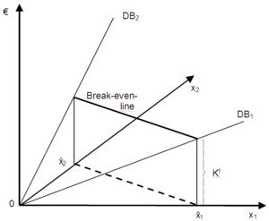
Other linear combinations enable fixed-cost-coverage in a similar way. Together, the corresponding break-even-points build a straight line between the break-even-corner-points, the break-even-line, as can be seen in the following three-dimensional graph (with x1 and x2 as horizontal axes and the profit, contribution and costs at the vertical axis.
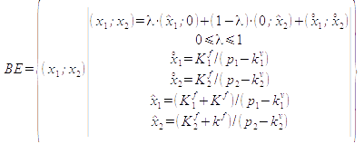
In order to facilitate algebraic formulations, we introduce the price vector (p1, p2), the variable cost vector (kv1, kv2), the unit contribution vector (d1, d2) and the output vector (x1, x2). The break-even-line is defined by the following output vector:
The case of two products with individual and joint fixed costs
Sometimes, cost-volume-profit analysis has to cope both with individual and joint fixed costs. Typical examples are multi-stage production processes: Computers are often manufactured for global customers in a single plant (with joint fixed costs) and customized to local specifications (power plugs, manuals, packaging, …) in local facilities. Movie production requires a large joint cost block to get the director’s cut, but finishing, translating, synchronization, subtitles and marketing are done separately for different countries or languages and cause individual fixed costs.
In our two-product case, we introduce Kf1 and Kf2 to capture the individual (or direct) fixed costs of products 1 and 2 and get the following break-even-form:
- (p1-kv1) · x1 + (p2-kv2) · x2 = d1 · x1 + d2 · x2 ≥ Kf + Kf1 + Kf2
Obviously, we only accept output-quantities x1 and x2 that cover their individual fixed costs. Thus, the individual break-even-conditions hold too:
- d1 · x1 ≥ Kf1
- d2 · x2 ≥ Kf2
This results in the condition:
- x1 ≥ x1 = Kf/d1
- x2 ≥ x1 = Kf/d2
The solution of the two individual conditions results in two break-even-points ![]() and
and ![]() . Considering too for the joint fixed cost leads to two break-even-corner-points
. Considering too for the joint fixed cost leads to two break-even-corner-points ![]() and
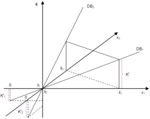
and ![]() . The possible break-even-points lie on the line between these corner-points. The graphical presentation of this case is similar to the previous case without individual fixed costs. However, we adjust the horizontal axes (x1 and x2) for the units that are necessary to cover the individual fixed costs.
. The possible break-even-points lie on the line between these corner-points. The graphical presentation of this case is similar to the previous case without individual fixed costs. However, we adjust the horizontal axes (x1 and x2) for the units that are necessary to cover the individual fixed costs.
In a formal way this break-even-line is captured by the set:
Note, that different to the previous case without individual fixed costs (and different to the formula proposed in Schweitzer/Troßmann (1998, p. 177), in this case the set of break-even-points is not just a linear combination of the two break-even-corner-points![]() and
and ![]() . Instead, it still is a linear combination of the break-even-points
. Instead, it still is a linear combination of the break-even-points ![]() and
and ![]() , corresponding to the joint fixed costs, plus the units
, corresponding to the joint fixed costs, plus the units ![]() and
and ![]() necessary to cover the individual fixed costs.
necessary to cover the individual fixed costs.
Analysis of the two-product case with restrictions
If our production process suffers from limited capacity (for example limited availability of inputs, limited market demand for some products, and so on), not all of the points on the break-even-line presented in the unrestricted case are feasible. For our product analysis it is important whether each product has a specific capacity constraint (individual restrictions) or whether one or several capacity constraints affect several products simultaneously (joint restrictions).
Individual restrictions are rather easy to handle. A direct restriction Bj to the volume of product j (caused for example by limited market size) can be amended to the break-even-line-set. The same is possible if we face an indirect constraint Bij of factor i (for example skilled labour) for product j. In this case, a production coefficient aij can capture the relation between product volume and necessary labor. The corresponding restrictions are:
- xj ≤ Bj or
- xj ≤ Bj/aij.
To be sure, for aij = 1, the former case is the same as the latter.
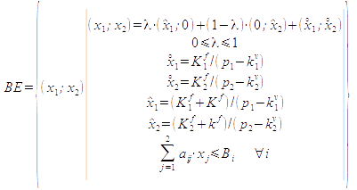
Joint restrictions are more difficult to handle. They occur if several products need the same, limited input factors or try to sell at the same market. In the linear case, with limitational production factors, the sum of inputs i needed for the several products j has to stay below the available capacity Bi. Since this is the general case which covers the former cases with direct or indirect product-specific restrictions too, the set of break-even-points is given just for this case.
Using vector notation for the capacity restraint, he set of break-even-points is:
The multi-product case
Since we are familiar with the two-product case, it is straightforward to generalize it to the multi-product case with n products (j = 1, …, J). Using again the unit prices pj, the variable costs kvj, the product-related fixed costs Kfj and joint fixed costs Kf, and the capacity constraints Bi and production coefficients aij, we get the following set of break-even-points in the multi-product case with joint restrictions.
A break-even-line consists of the possible quantities of two products which cover joint fixed costs and linear sales revenue and variable cost functions. In the case of three products we get a break-even-plane. The combinations of four or more products result in break-even-hyper-planes which are difficult to present graphically. For such cases, the analysis is restricted to the vector form of the set of break-even-points (as presented above; and in more detail by Schweitzer/Troßmann (1998, pp. 173 ff.; 203 ff.) or Schweitzer/Troßmann/Lawson (1992), Chapter 4).
Evaluation of explicit multi-product break-even-analyses
A large number of managerial decisions deal with multi-product or similar problems (for example product or regional market differentiation, or aiming at economies of scope). They combine both individual and joint production processes, and hence, cost. In many cases, the exact outputs of those products or volumes of the markets are unknown. Thus, a break-even-model that provides information about critical outputs or market volumes, is useful. Break-even-corner-points and intuitive graphical representations of the cost-volume-profit-problem support the decision making processes and controlling and offer valuable additional information compared to the simplifying use of single-product or single-index break-even approaches. However, the more products we include in the analysis, the more contingent are our break-even-hyper-planes. Whether a certain quantity of a product is sufficient or not, depends on the outputs of (too) many other products. In such situations, other approaches may provide better guidelines for decision-making. Apart from the simplifying break-even-analyses already mentioned, this could be the identification of typical output combinations and the calculation of their profit.
---
References:
Break-even-Analyse
Multi-product break-even-analysis
Accounting exercises 4: Break-even-Analysis
Schweitzer, M.; E. Troßmann; G. E. Lawson: Break-even-Analyses. John Wiley & Sons 1992.
Schweitzer, M.; E. Troßmann: Break-even-Analysen. 2. Aufl., Berlin 1998 (1. Aufl. 1986).
